NCAA Football Coach Salary Recommendation Project
NCAA FOOTBALL SALARY RECOMMENDATIONS
The purpose of this case study is to take real world data and provide insight, understanding and wisdom to a decision maker. In this case specifically we are dealing with the salaries of NCAA Division I Football Coaches. We are exploring how we can recommend the best salary for Syracuse University's head football coach? First, lets Import the packages we will be using:
# import packages for analysis and modeling
import pandas as pd #data frame operations
import numpy as np #arrays and math functions
from scipy.stats import uniform #for training and test splits
import statsmodels.api as sm  # statistical models (including regression)
import statsmodels.formula.api as smf  # R-like model specification
import matplotlib.pyplot as plt #2D plotting
import seaborn as sns #seaborn for plotting
from sklearn.linear_model import LinearRegression
from sklearn.metrics import mean_squared_error
from sklearn.metrics import r2_score
Data Preparation
While we were supplied a coaches dataset to work with initially, this did not provide all the data needed to provide a thorough analysis. The following for data sets were combined to give us the information needed:
- Coaches data – 2014 coaches data set provided containing school, conference, coach and various types of pay (school pay, total pay, bonus, bonus paid, assistant pay, buyout)
- Stadium capacity data – data scraped from www.collegegridirons.com containing stadium name, school, conference, capacity, and year opened
- Graduation rates – 2012-2013 school year graduation reates obrainted from the NCAA containing borth GSR and FGR. 2006 cohort graduation rates were used. Contains Year, School. Conference, Sport, State, GSR, FGR
- Win Loss Record – Win Loss record for last year (2019) scrapped from www.teamrankings.com
Coaches Data
The initial dataset was supplied to us and is stored in my git repository which was inported into a dataframe. A quick computation of some of the descriptive statistics show that there were 129 total entries (all unique) for school names beloning to 11 unique conferences. In addition we see the count and unique entries for all the columns in the dataset. I also checked for null values and found nine in the dataframe
        School Conference              Coach  ... BonusPaid AssistantPay Buyout
count      129        129                129  ...       129          129    129
unique     129         11                129  ...        51            1    102
top     Hawaii    Big Ten  Bronco Mendenhall  ...        --          $0      --
freq         1         14                  1  ...        41          129     22

[4 rows x 9 columns]
********************************************************************************
Are there any null values? False
********************************************************************************
Columns with null values:
 School          0
Conference      0
Coach           0
SchoolPay       0
TotalPay        0
Bonus           0
BonusPaid       0
AssistantPay    0
Buyout          0
dtype: int64
Number of observations:
 129
A quick look at the head of the dataframe shows us the first 5 rows. We see School, Conference, Coach, SchoolPay, TotalPay, Bonus, BonusPaid, AssistantPay and Buyout. The fist thing we notice is that the dollar amounts are objects which will need to be covereted into mueric format.
coaches.head()
| School | Conference | Coach | SchoolPay | TotalPay | Bonus | BonusPaid | AssistantPay | Buyout | |
|---|---|---|---|---|---|---|---|---|---|
| 0 | Air Force | Mt. West | Troy Calhoun | 885000 | 885000 | 247000 | -- | $0 | -- |
| 1 | Akron | MAC | Terry Bowden | $411,000 | $412,500 | $225,000 | $50,000 | $0 | $688,500 |
| 2 | Alabama | SEC | Nick Saban | $8,307,000 | $8,307,000 | $1,100,000 | $500,000 | $0 | $33,600,000 |
| 3 | Alabama at Birmingham | C-USA | Bill Clark | $900,000 | $900,000 | $950,000 | $165,471 | $0 | $3,847,500 |
| 4 | Appalachian State | Sun Belt | Scott Satterfield | $712,500 | $712,500 | $295,000 | $145,000 | $0 | $2,160,417 |
Our dollar amounts are actually stored as astrings so I ran a function to convert them to numeric values and reinspected.
# Clean up: convert dollar amounts from object to numeric
coaches.head()
| School | Conference | Coach | SchoolPay | TotalPay | Bonus | BonusPaid | AssistantPay | Buyout | |
|---|---|---|---|---|---|---|---|---|---|
| 0 | Air Force | Mt. West | Troy Calhoun | 885000.0 | 885000.0 | 247000.0 | 0.0 | 0.0 | 0.0 |
| 1 | Akron | MAC | Terry Bowden | 411000.0 | 412500.0 | 225000.0 | 50000.0 | 0.0 | 688500.0 |
| 2 | Alabama | SEC | Nick Saban | 8307000.0 | 8307000.0 | 1100000.0 | 500000.0 | 0.0 | 33600000.0 |
| 3 | Alabama at Birmingham | C-USA | Bill Clark | 900000.0 | 900000.0 | 950000.0 | 165471.0 | 0.0 | 3847500.0 |
| 4 | Appalachian State | Sun Belt | Scott Satterfield | 712500.0 | 712500.0 | 295000.0 | 145000.0 | 0.0 | 2160417.0 |
Webscraping Stadium Capacity Data
Syed Nazrul has a great Webscraping tutorial he created on you tube using pokemon data which you can see visit below
PokeScrape 1: Scraping an online PokeDex (Pokemon data) with Python
I went to the College Gridirons Website and scrapped data on college football stadiums by capacity. This data included the Stadium Name, The College, Conference, Capacity and the year it opened. Once scrapped, the data required extensive cleaned up and once completed it was stored in a new dataframe.
# create Stadiums df
stadiums.head()
| Stadium | School | Conference | Capacity | Opened | |
|---|---|---|---|---|---|
| 58 | Falcon Stadium | Air Force | Mountain West | 52237.0 | 1962 |
| 107 | InfoCision Stadium | Akron | MAC | 30000.0 | 2009 |
| 5 | Bryant Denny Stadium | Alabama | SEC | 101821.0 | 1929 |
| 118 | Kidd Brewer Stadium | Appalachian State | Sun Belt | 24150.0 | 1962 |
| 50 | Arizona Stadium | Arizona | Pac 12 | 56037.0 | 1928 |
Import Graduation Rates Data
From Bleacher report September 4, 2013
https://bleacherreport.com/articles/1731218-college-football-schools-with-the-best-and-worst-graduation-rates#slide0
-
FGR - Federal Graduation Rate - This method keeps track of first-time freshmen who are full-time students. It follows those students over the course of a six-year period to see if they graduate at the same institution at which they began their secondary education. This method does not account for students who transfer.
-
GSR - Graduation Success Rate - Uses the same type of data as the FGR, but the GSR data also takes into account students who transfer into a school and graduate from that same school. It also doesn’t count against a school’s rate when a student-athlete in good standing transfers out of that institution to attend another.
The 2013 Graduation Rate data was obtained using the 2006 cohort graduation rates for both GSR and FGR. There was some clean up required to ensure that the school names matched the entries in the original coaches dataset. For example, US Naval Academy was listed as Navy in the coaches set.
# import graduation rate data
# obtained from https://web3.ncaa.org/aprsearch/gsrsearch
# Sport = Football, Year = 2012-2013
gradrates.head()
| Cohort Year | School | Conference | Sport | State | GSR | FGR | |
|---|---|---|---|---|---|---|---|
| 210 | 2006 | Air Force | Mountain West Conference | Football | CO | 93 | NaN |
| 0 | 2006 | Akron | Mid-American Conference | Football | OH | 58 | 52.0 |
| 3 | 2006 | Alabama | Southeastern Conference | Football | AL | 73 | 57.0 |
| 1 | 2006 | Alabama A&M | Southwestern Athletic Conf. | Football | AL | 40 | 45.0 |
| 2 | 2006 | Alabama State | Southwestern Athletic Conf. | Football | AL | 81 | 59.0 |
Win Loss Record
2019 Win-Loss Record was scrapped from the website www.teamrankings.com and a new dataframe was created. This data also required extensive cleanup to ensure the school names match and was then stored in its own dataframe.
#Scrape 2019 Win-Loss Records
#create url
url='https://www.teamrankings.com/ncf/trends/win_trends/?range=yearly_2019'
WinLoss.head()
| School | Win-Loss Record2019 | WinPercentage2019 | MOV | ATS | WinPer2019 | |
|---|---|---|---|---|---|---|
| 9 | Air Force | 11-2-0 | 84.6% | 14.2 | +5.7 | 0.846 |
| 129 | Akron | 0-12-0 | 0.0% | -25.8 | -11.6 | 0.000 |
| 14 | Alabama | 11-2-0 | 84.6% | 28.6 | +0.6 | 0.846 |
| 2 | Appalachian State | 13-1-0 | 92.9% | 18.8 | +4.9 | 0.929 |
| 108 | Arizona | 4-8-0 | 33.3% | -8.8 | -5.5 | 0.333 |
All the data has now been obtained and was merged into one dataframe which I named "finalcoaches" consisting of the coaches, gradrates, stadium capacity and win-loss record sets. The sets were merged on School Name.
# Merge all dfs to create finalcoaches
merge1 = coaches.merge(stadiums, on='School', how='left') #Add stadium data to coaches, match on School to create merge1
merge2 = merge1.merge(gradrates, on='School', how='left') #Add gradrates data to merge1, match on School to create merge2
finalcoaches = merge2.merge(WinLoss, on='School', how='left') #Add WinLoss data to merge2, match on School to create finalcoaches

#drop uneeded columns
finalcoaches = finalcoaches.drop(['Stadium', 'Conference_y', 'Conference',
                                  'Sport',
                                  'Opened','MOV','ATS'], axis=1)

# rename
finalcoaches.rename(columns={'Conference_x':'Conference'}, inplace=True)

# using apply function to create a new column for graphing purposes (thousands)
finalcoaches['TotalPayThousands'] = finalcoaches.apply(lambda row: (row.TotalPay * 0.001), axis = 1)

# compute descriptive statistics for original variables
print(finalcoaches.describe())
print("*"*80)
print(finalcoaches.head())
          SchoolPay      TotalPay  ...  WinPer2019  TotalPayThousands
count  1.290000e+02  1.290000e+02  ...  129.000000         129.000000
mean   2.335563e+06  2.342113e+06  ...    0.521217        2342.113140
std    1.898654e+06  1.903114e+06  ...    0.217709        1903.113765
min    0.000000e+00  0.000000e+00  ...    0.000000           0.000000
25%    7.625700e+05  7.625700e+05  ...    0.333000         762.570000
50%    1.800000e+06  1.830000e+06  ...    0.538000        1830.000000
75%    3.550000e+06  3.550000e+06  ...    0.643000        3550.000000
max    8.307000e+06  8.307000e+06  ...    1.000000        8307.000000

[8 rows x 12 columns]
********************************************************************************
                  School Conference  ... WinPer2019  TotalPayThousands
0              Air Force   Mt. West  ...      0.846              885.0
1                  Akron        MAC  ...      0.000              412.5
2                Alabama        SEC  ...      0.846             8307.0
3  Alabama at Birmingham      C-USA  ...      0.643              900.0
4      Appalachian State   Sun Belt  ...      0.929              712.5

[5 rows x 18 columns]
Upon review, it is observed that there are some null values from the stadium capacity and win record data. We will now take a look at these rows for further investigation.
#check for null values in the dataframe
are_null_values = finalcoaches.isnull().values.any()
num_nulls = finalcoaches.isnull().sum()
print("*"*80)
print("Are there any null values?",are_null_values)
print("*"*80)
print("Columns with null values: ",num_nulls)
print("Number of observations: ",len(finalcoaches))
********************************************************************************
Are there any null values? True
********************************************************************************
Columns with null values:  School                 0
Conference             0
Coach                  0
SchoolPay              0
TotalPay               0
Bonus                  0
BonusPaid              0
AssistantPay           0
Buyout                 0
Capacity               1
Cohort Year            4
State                  4
GSR                    4
FGR                    8
Win-Loss Record2019    0
WinPercentage2019      0
WinPer2019             0
TotalPayThousands      0
dtype: int64
Number of observations:  129
There were 8 total schools missing FGR, 4 of which were also missing their GSR. Since we have more data for GSR we will use that information rather than the FGR. In addition, I believe this is the rate we should use as this is the method the NCAA is currently using to evaluate graduation rates. The schools missing the GSR values would be dropped from the set.
# Schools missing FGR (Federal Graduation Rate) and GSR (Graduate Success Rate)
finalcoaches[finalcoaches['FGR'].isna()]
| School | Conference | Coach | SchoolPay | TotalPay | Bonus | BonusPaid | AssistantPay | Buyout | Capacity | Cohort Year | State | GSR | FGR | Win-Loss Record2019 | WinPercentage2019 | WinPer2019 | TotalPayThousands | |
|---|---|---|---|---|---|---|---|---|---|---|---|---|---|---|---|---|---|---|
| 0 | Air Force | Mt. West | Troy Calhoun | 885000.0 | 885000.0 | 247000.0 | 0.0 | 0.0 | 0.0 | 52237.0 | 2006.0 | CO | 93.0 | NaN | 11-2-0 | 84.6% | 0.846 | 885.000 |
| 9 | Army | Ind. | Jeff Monken | 932521.0 | 932521.0 | 0.0 | 0.0 | 0.0 | 0.0 | 38000.0 | 2006.0 | NY | 89.0 | NaN | 5-8-0 | 38.5% | 0.385 | 932.521 |
| 21 | Charlotte | C-USA | Brad Lambert | 625000.0 | 625000.0 | 120000.0 | 0.0 | 0.0 | 556389.0 | 15314.0 | NaN | NaN | NaN | NaN | 7-6-0 | 53.8% | 0.538 | 625.000 |
| 38 | Georgia State | Sun Belt | Shawn Elliott | 569000.0 | 569000.0 | 220000.0 | 60000.0 | 0.0 | 1500000.0 | 23000.0 | NaN | NaN | NaN | NaN | 7-6-0 | 53.8% | 0.538 | 569.000 |
| 69 | Navy | AAC | Ken Niumatalolo | 2163000.0 | 2163000.0 | 0.0 | 0.0 | 0.0 | 0.0 | 34000.0 | 2006.0 | MD | 84.0 | NaN | 11-2-0 | 84.6% | 0.846 | 2163.000 |
| 85 | Old Dominion | C-USA | Bobby Wilder | 654667.0 | 654667.0 | 504895.0 | 0.0 | 0.0 | 1200000.0 | 20118.0 | 2006.0 | VA | 50.0 | NaN | 1-11-0 | 8.3% | 0.083 | 654.667 |
| 95 | South Alabama | Sun Belt | Steve Campbell | 600000.0 | 600000.0 | 295000.0 | 0.0 | 0.0 | 918333.0 | 40646.0 | NaN | NaN | NaN | NaN | 2-10-0 | 16.7% | 0.167 | 600.000 |
| 110 | Texas-San Antonio | C-USA | Frank Wilson | 1100000.0 | 1100000.0 | 185000.0 | 17500.0 | 0.0 | 3562500.0 | 65000.0 | NaN | NaN | NaN | NaN | 4-8-0 | 33.3% | 0.333 | 1100.000 |
Since total pay was converted into numerical values, I looked for all schools where the total pay was listed as "0". The 4 schools with no listed total pay would be dropped from the set.
# Schools missing TotalPay
finalcoaches.loc[finalcoaches['TotalPay'] == 0]
| School | Conference | Coach | SchoolPay | TotalPay | Bonus | BonusPaid | AssistantPay | Buyout | Capacity | Cohort Year | State | GSR | FGR | Win-Loss Record2019 | WinPercentage2019 | WinPer2019 | TotalPayThousands | |
|---|---|---|---|---|---|---|---|---|---|---|---|---|---|---|---|---|---|---|
| 12 | Baylor | Big 12 | Matt Rhule | 0.0 | 0.0 | 0.0 | 0.0 | 0.0 | 0.0 | 45140.0 | 2006.0 | TX | 67.0 | 48.0 | 11-3-0 | 78.6% | 0.786 | 0.0 |
| 16 | Brigham Young | Ind. | Kalani Sitake | 0.0 | 0.0 | 0.0 | 0.0 | 0.0 | 0.0 | 63725.0 | 2006.0 | UT | 57.0 | 42.0 | 7-6-0 | 53.8% | 0.538 | 0.0 |
| 91 | Rice | C-USA | Mike Bloomgren | 0.0 | 0.0 | 0.0 | 0.0 | 0.0 | 0.0 | 47000.0 | 2006.0 | TX | 96.0 | 89.0 | 3-9-0 | 25.0% | 0.250 | 0.0 |
| 99 | Southern Methodist | AAC | Sonny Dykes | 0.0 | 0.0 | 0.0 | 0.0 | 0.0 | 0.0 | 32000.0 | 2006.0 | TX | 75.0 | 63.0 | 10-3-0 | 76.9% | 0.769 | 0.0 |
Lastly I looked at schools where the stadium capacity was not listed. Only one school was missing the capacity value, which was dropped from the dataset.
# Schools missing Stadium Capacity
finalcoaches[finalcoaches['Capacity'].isna()]
| School | Conference | Coach | SchoolPay | TotalPay | Bonus | BonusPaid | AssistantPay | Buyout | Capacity | Cohort Year | State | GSR | FGR | Win-Loss Record2019 | WinPercentage2019 | WinPer2019 | TotalPayThousands | |
|---|---|---|---|---|---|---|---|---|---|---|---|---|---|---|---|---|---|---|
| 51 | Liberty | Ind. | Turner Gill | 947281.0 | 947281.0 | 0.0 | 0.0 | 0.0 | 0.0 | NaN | 2006.0 | VA | 65.0 | 54.0 | 8-5-0 | 61.5% | 0.615 | 947.281 |
#Cleanup

# Drop all schools with 0 TotalPay
finalcoaches = finalcoaches.drop(finalcoaches.index[finalcoaches.TotalPay == 0])
# DROP GSR null
finalcoaches = finalcoaches.dropna(axis=0, subset=['GSR'])
# DROP missing Stadium Capacity
finalcoaches = finalcoaches.dropna(axis=0, subset=['Capacity'])
Power 5 Conferences
I also decided to add a column to our final dataframe indicating whether or not the school was a member of the "Power5" conferences. I suspected that these conferences had a significantly higher pay than the other conferences as they would want to recruit the top football coaches for their schools.
In college football, the term Power Five conferences refers to five athletic conferences whose
members are part of the Football Bowl Subdivision (FBS) of NCAA Division I, the highest level
of collegiate football in the United States. The conferences are:
the Atlantic Coast Conference (ACC), Big Ten Conference, Big 12 Conference,
Pac-12 Conference, and Southeastern Conference (SEC).
The term "Power Five" is not defined by the National Collegiate Athletic Association (NCAA),
and the origin of the term is unknown. It has been used in its current meaning since at least 2006.
Descriptive Visualizations
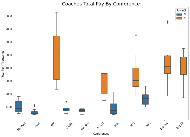
First I decided to create a boxplot of total pay by conference as I suspected there were some major differences. In addition, I added "Power5" as a hue to see if there was a differene between the conferences belonging to the Power5 and the remaining conferences.
Our first observation is that the median total pay for the Power5 are higher than the remaining conferences. We see that their median amount is higher than the maximum for all other conferences.
# Create Boxplots By Conference
coachesbox = sns.boxplot(x="Conference",
                         y="TotalPayThousands",
                         data=finalcoaches,
                         hue="Power5")

#add title, xlabel and y label
plt.title('Coaches Total Pay By Conference', fontsize = 18)
plt.xlabel('Conferences')
plt.ylabel('Total Pay (Thousands)')
#rotate day of week (dow) names to reduce overlap
coachesbox.set_xticklabels(coachesbox.get_xticklabels(),rotation=45)
plt.show()
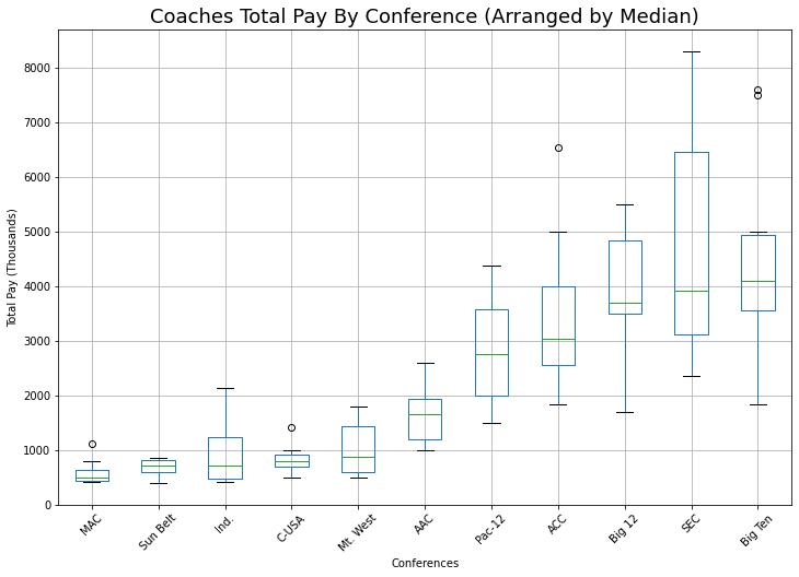
When arranged by median TotalPay, we see the top 5 schools are all members of the Power5, in ascending order Pac-12, ACC, Big12, SEC, Big10. I was expecting the SEC to have higher numbers than all the other conferences based on the strength of this conference. It had the highest maximum, minimum and upper quartile of all the conferences. It's lower quartile was lower than the Big 12's and Big Ten. It's medium is lower than the Big Ten's.
One thing to note is that the 6th school on the list (be median) is the AAC (The American), which was known as the Big East prior to the 2010-2014 NCAA Conference Realignment. The Big East was the part of the original sex college power confereces of the Bowl Championshop Series (BCS).
#https://stackoverflow.com/questions/21912634/how-can-i-sort-a-boxplot-in-pandas-by-the-median-values

def boxplot_sorted(df, by, column):
  df2 = pd.DataFrame({col:vals[column] for col, vals in df.groupby(by)})
  meds = df2.median().sort_values(ascending=True)
  df2[meds.index].boxplot(rot=45)

boxplot_sorted(finalcoaches, by=["Conference"], column="TotalPayThousands")
plt.title('Coaches Total Pay By Conference (Arranged by Median)', fontsize = 18)
plt.xlabel('Conferences')
plt.ylabel('Total Pay (Thousands)')
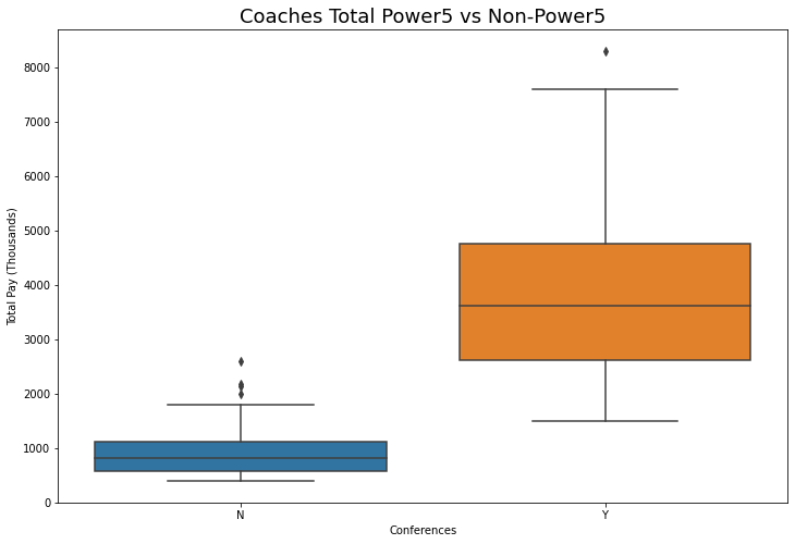
When comparing Power5 vs Non-Power5, we see that there is a significant higher TotalPay for the Power5 conferences. The minimum TotalPay is lower than the maximum, however we see that all other measures of statistical distribution for the Power 5 schools are higher than the maximum Total Pay of the non-Power5 schools.
# Create Boxplots By Conference
coachesbox2 = sns.boxplot(x="Power5",
                         y="TotalPayThousands",
                         data=finalcoaches
                         )

#add title, xlabel and y label
plt.title('Coaches Total Power5 vs Non-Power5', fontsize = 18)
plt.xlabel('Conferences')
plt.ylabel('Total Pay (Thousands)')
#rotate day of week (dow) names to reduce overlap
coachesbox.set_xticklabels(coachesbox.get_xticklabels(),rotation=45)
plt.show()
I also created a correlation matrix to see what relationships we could find between the variables. I settled on the variables Capacity, GSR, WinPercentage2019(WinPer2019), and all the Conference variables. We see that Capacity has the highest correlation and has the biggest effect on Total Pay (positive). We also see that GSR, WinPer2019, as well as the 5 elite schools have a positive effect on Pay, with the SEC conference having the biggest effect. Notice that the non-Power5 all have a negative effect on pay.
# Check Correlation Matrix
coachescorr = finalcoaches.drop(['AssistantPay', 'Cohort Year', 'SchoolPay', 'Bonus', 'BonusPaid',
                                 'Buyout', 'TotalPayThousands', 'FGR'], axis=1)
# create corr df
corr = coachescorr.corr()

# Generate a mask for the upper triangle
mask = np.zeros_like(corr, dtype=np.bool)
mask[np.triu_indices_from(mask)] = True

# Print heatmap
plt.figure(figsize=(12,8))
sns.heatmap(coachescorr.corr(), mask=mask,annot = True, vmin=-1, vmax=1, center= 0, cmap= 'coolwarm',
           linewidths=.5 #, linecolor='black'
           )
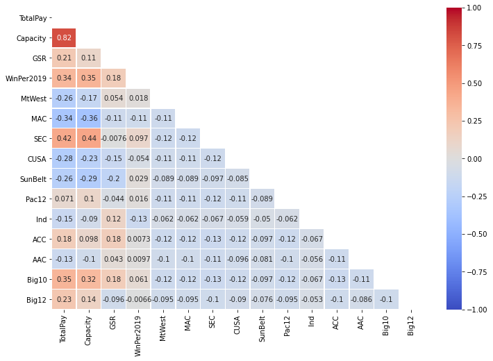
I wanted to ignore the conferences for a second and look at just Capacity, GSR and Win Percentage to see what relationship existed between them and TotalPay. We see that there is definitely a positive relationship between TotalPay and Capacity but it is harder to tell with GSR and Win Percentage.
# Plot Total Pay vs Capacity, GSR, Win Percentage(2019)
# visualize the relationship between the features and the response using scatterplots
g=sns.pairplot(finalcoaches, x_vars=['Capacity','GSR','WinPer2019'],
             y_vars='TotalPay', height=4, aspect=1, kind='reg'
              )
#plt.title('Total Pay vs. Capacity, GSR, 2019 Win Percentage', y=4, fontsize = 16)
plt.subplots_adjust(top=.85)
g.fig.suptitle('Total Pay vs. Capacity, GSR, 2019 Win Percentage',fontsize = 18)
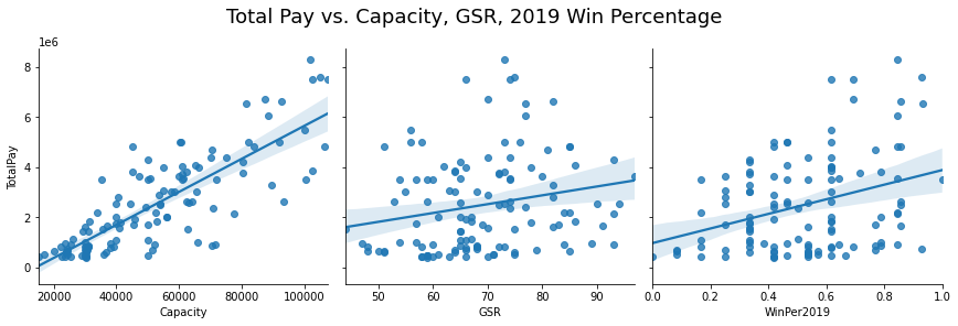
Although I was not looking at specific conferences, I still wanted to see if being a member of the Power5 played a role and plotted the points again with distinction between the two. When we use that distinction to color the points on the graph we see some patterns that weren’t as apparent in the previous plot.
In the Capacity graph, I notice that although there is an overall increase, the rate at which they occur is not the same across schools as evident by the slopes of the two lines. We see a similar scenario play out when it comes to WinPercentage. What this tells me, is that win percentage as well as stadium capacity have a larger effect on the Power5 football conference school’s total pay, when compared to the non-Power5 conference schools. For GSR, we see that the slopes are similar. We see that yes, there is an increase in TotalPay, albeit minor. In laymen’s terms what we are seeing is this, Winning percentage and Stadium size play a larger role in a Coach's pay than graduation rates do.
# Plot Total Pay vs Capacity, GSR, Win Percentage(2019)
# visualize the relationship between the features and the response using scatterplots
g=sns.pairplot(finalcoaches, x_vars=['Capacity','GSR','WinPer2019'], hue="Power5",
             y_vars='TotalPay', height=4, aspect=1, kind='reg'
              )
#plt.title('Total Pay vs. Capacity, GSR, 2019 Win Percentage', y=4, fontsize = 16)
plt.subplots_adjust(top=.85)
g.fig.suptitle('Total Pay vs. Capacity, GSR, 2019 Win Percentage',fontsize = 18)

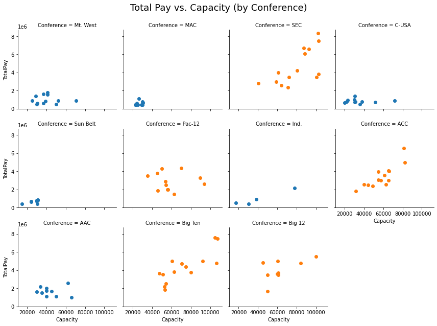
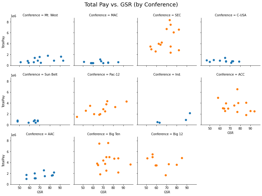
I also replicated this graph using facet grids by conference. For the most part the faceted grids behaved similarly to the grouped versions above.
For Total Pay vs Capacity, most conferences had a positive relationship between the two, but we see steeper slopes for the Power5 schools. It was difficult to see the relatinship for Mt West, MAC and Pac-12
#print("Total Pay vs. Capacity by Conference")
g = sns.FacetGrid(finalcoaches, col="Conference", col_wrap=4, hue="Power5", )
g.map(plt.scatter, "Capacity","TotalPay", alpha=1);
plt.subplots_adjust(top=0.9)
g.fig.suptitle('Total Pay vs. Capacity (by Conference)',fontsize = 18)
For Total Pay vs GSR, we also see positive relationships for most of the schools with there being a significant slope difference in the Power5. It was difficult to see a pattern for the Big Ten.
There was one particular pattern here that I thought was interesting. It seems that for the ACC and Big 12, as graduation rates increased the TotalPay actually went down which didnt match my inital expectations. I wondered if the reason for this had to do with the relationship between graduation rates and wins, which was slightly positive in the correlation matrix (0.18)? Maybe there were some schools that lost some of their good players due to academics and it impacted their winning percentage? Potentially, a losing record could lead to a coach replacement and maybe offering a higher salary to recruit a better coach?
#print("Total Pay vs. GSR by Conference")
g = sns.FacetGrid(finalcoaches, col="Conference", col_wrap=4, hue="Power5")
g.map(plt.scatter, "GSR","TotalPay", alpha=1);
plt.subplots_adjust(top=0.9)
g.fig.suptitle('Total Pay vs. GSR (by Conference)',fontsize = 18)
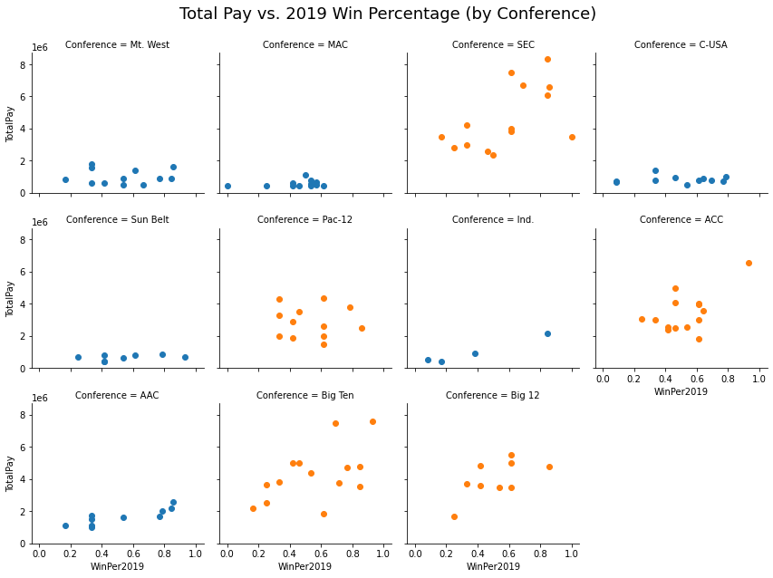
For Total Pay vs WinPercentage, most conferences had a positive relationship between the two, but we see steeper slopes for the Power5 schools. It was difficult to see the relatinship for Pac-12
#print("Total Pay vs. Win Percentage by Conference")
g = sns.FacetGrid(finalcoaches, col="Conference", col_wrap=4, hue="Power5")
g.map(plt.scatter, "WinPer2019","TotalPay", alpha=1);
plt.subplots_adjust(top=0.9)
g.fig.suptitle('Total Pay vs. 2019 Win Percentage (by Conference)',fontsize = 18)
Model Creation
I will create a model using the ordinarly least sums (OLS) method for simple lenear regression. First, let me create my test and training sets, 2/3 for training and 1/3 for testing.
# employ training-and-test regimen for model validation
np.random.seed(1234)
finalcoaches['runiform'] = uniform.rvs(loc = 0, scale = 1, size = len(finalcoaches))
finalcoaches_train = finalcoaches[finalcoaches['runiform'] >= 0.33]
finalcoaches_test = finalcoaches[finalcoaches['runiform'] < 0.33]
********************************************************************************

finalcoaches_train data frame (rows, columns):  (86, 31)
********************************************************************************
                  School Conference              Coach  ...  Big10  Big12  runiform
1                  Akron        MAC       Terry Bowden  ...      0      0  0.622109
2                Alabama        SEC         Nick Saban  ...      0      0  0.437728
3  Alabama at Birmingham      C-USA         Bill Clark  ...      0      0  0.785359
4      Appalachian State   Sun Belt  Scott Satterfield  ...      0      0  0.779976
7               Arkansas        SEC        Chad Morris  ...      0      0  0.801872

[5 rows x 31 columns]
********************************************************************************

finalcoaches_test data frame (rows, columns):  (34, 31)
********************************************************************************
             School Conference           Coach  ...  Big10  Big12  runiform
0         Air Force   Mt. West    Troy Calhoun  ...      0      0  0.191519
5           Arizona     Pac-12    Kevin Sumlin  ...      0      0  0.272593
6     Arizona State     Pac-12    Herm Edwards  ...      0      0  0.276464
19  Central Florida        AAC     Josh Heupel  ...      0      0  0.013768
25         Colorado     Pac-12  Mike MacIntyre  ...      0      0  0.075381

[5 rows x 31 columns]
Model 1: With Conference + Capacity + WinPer2019 + GSR
The first model I created would test the effect Conference, Stadium Capacity, 2019 WIn Percentage and Graduation Rate (GSR) had on the total pay.
# specify a simple model with Team Conference
conference_model = str('TotalPay ~ SEC + CUSA + SunBelt + Pac12 + Ind + ACC + AAC + Big10 + Big12 + MtWest + MAC + Capacity + WinPer2019 + GSR')
                            OLS Regression Results
==============================================================================
Dep. Variable:               TotalPay   R-squared:                       0.810
Model:                            OLS   Adj. R-squared:                  0.776
Method:                 Least Squares   F-statistic:                     23.60
Date:                Sat, 11 Apr 2020   Prob (F-statistic):           7.22e-21
Time:                        19:37:51   Log-Likelihood:                -1295.2
No. Observations:                  86   AIC:                             2618.
Df Residuals:                      72   BIC:                             2653.
Df Model:                          13
Covariance Type:            nonrobust
==============================================================================
                 coef    std err          t      P>|t|      [0.025      0.975]
------------------------------------------------------------------------------
Intercept  -1.591e+06   7.73e+05     -2.059      0.043   -3.13e+06   -5.08e+04
SEC         1.175e+06   3.59e+05      3.271      0.002    4.59e+05    1.89e+06
CUSA       -8.397e+05   2.87e+05     -2.927      0.005   -1.41e+06   -2.68e+05
SunBelt    -6.237e+05   3.74e+05     -1.669      0.100   -1.37e+06    1.21e+05
Pac12       3.165e+05   3.23e+05      0.979      0.331   -3.28e+05    9.61e+05
Ind        -1.785e+06   6.74e+05     -2.649      0.010   -3.13e+06   -4.42e+05
ACC         4.487e+05   3.16e+05      1.422      0.159    -1.8e+05    1.08e+06
AAC        -4.176e+05   3.43e+05     -1.217      0.228    -1.1e+06    2.66e+05
Big10       6.661e+05   3.86e+05      1.726      0.089   -1.03e+05    1.44e+06
Big12       1.087e+06   5.19e+05      2.095      0.040    5.28e+04    2.12e+06
MtWest     -9.013e+05   3.24e+05     -2.778      0.007   -1.55e+06   -2.55e+05
MAC        -7.173e+05   3.18e+05     -2.255      0.027   -1.35e+06   -8.31e+04
Capacity      41.6164      7.175      5.800      0.000      27.314      55.919
WinPer2019  9.855e+05   5.38e+05      1.831      0.071   -8.74e+04    2.06e+06
GSR         2.083e+04   1.07e+04      1.944      0.056    -527.530    4.22e+04
==============================================================================
Omnibus:                        1.269   Durbin-Watson:                   1.745
Prob(Omnibus):                  0.530   Jarque-Bera (JB):                0.843
Skew:                           0.230   Prob(JB):                        0.656
Kurtosis:                       3.156   Cond. No.                     1.12e+18
==============================================================================

Warnings:
[1] Standard Errors assume that the covariance matrix of the errors is correctly specified.
[2] The smallest eigenvalue is 2.12e-25. This might indicate that there are
strong multicollinearity problems or that the design matrix is singular.
Model 2: Model 1 w/ no Conference
Model 2 would remove the conferences as variables to see if removing this variable had any significant difference.
# specify a simple model with Team Conference
elite_model = str('TotalPay ~ Capacity + WinPer2019 + GSR')
********************************************************************************
                            OLS Regression Results
==============================================================================
Dep. Variable:               TotalPay   R-squared:                       0.722
Model:                            OLS   Adj. R-squared:                  0.711
Method:                 Least Squares   F-statistic:                     70.81
Date:                Sat, 11 Apr 2020   Prob (F-statistic):           1.08e-22
Time:                        19:37:51   Log-Likelihood:                -1311.6
No. Observations:                  86   AIC:                             2631.
Df Residuals:                      82   BIC:                             2641.
Df Model:                           3
Covariance Type:            nonrobust
==============================================================================
                 coef    std err          t      P>|t|      [0.025      0.975]
------------------------------------------------------------------------------
Intercept   -2.49e+06    7.1e+05     -3.506      0.001    -3.9e+06   -1.08e+06
Capacity      65.4024      4.922     13.287      0.000      55.610      75.195
WinPer2019  2.604e+05   5.71e+05      0.456      0.649   -8.75e+05     1.4e+06
GSR         2.092e+04   1.01e+04      2.063      0.042     749.416    4.11e+04
==============================================================================
Omnibus:                        4.660   Durbin-Watson:                   2.057
Prob(Omnibus):                  0.097   Jarque-Bera (JB):                4.579
Skew:                          -0.304   Prob(JB):                        0.101
Kurtosis:                       3.953   Cond. No.                     3.58e+05
==============================================================================

Warnings:
[1] Standard Errors assume that the covariance matrix of the errors is correctly specified.
[2] The condition number is large, 3.58e+05. This might indicate that there are
strong multicollinearity or other numerical problems.
Model 3: Model 1 + State
Model 3 would add a state variable to model 1
# specify a simple model with Team Conference
state_model = str('TotalPay ~ Conference + Capacity + WinPer2019 + GSR + State')
********************************************************************************
                            OLS Regression Results
==============================================================================
Dep. Variable:               TotalPay   R-squared:                       0.910
Model:                            OLS   Adj. R-squared:                  0.813
Method:                 Least Squares   F-statistic:                     9.407
Date:                Sat, 11 Apr 2020   Prob (F-statistic):           2.18e-11
Time:                        19:37:51   Log-Likelihood:                -1263.1
No. Observations:                  86   AIC:                             2616.
Df Residuals:                      41   BIC:                             2727.
Df Model:                          44
Covariance Type:            nonrobust
==========================================================================================
                             coef    std err          t      P>|t|      [0.025      0.975]
------------------------------------------------------------------------------------------
Intercept              -1.837e+06   1.17e+06     -1.569      0.124    -4.2e+06    5.28e+05
Conference[T.ACC]       1.037e+06   5.94e+05      1.746      0.088   -1.63e+05    2.24e+06
Conference[T.Big 12]    9.164e+05   8.17e+05      1.121      0.269   -7.34e+05    2.57e+06
Conference[T.Big Ten]   1.494e+06   7.82e+05      1.910      0.063   -8.59e+04    3.07e+06
Conference[T.C-USA]    -9.452e+05   5.33e+05     -1.775      0.083   -2.02e+06     1.3e+05
Conference[T.Ind.]     -1.109e+06   1.02e+06     -1.085      0.284   -3.17e+06    9.56e+05
Conference[T.MAC]      -6.375e+05    6.6e+05     -0.966      0.340   -1.97e+06    6.95e+05
Conference[T.Mt. West] -1.117e+06   6.69e+05     -1.669      0.103   -2.47e+06    2.34e+05
Conference[T.Pac-12]   -4.127e+04    6.7e+05     -0.062      0.951   -1.39e+06    1.31e+06
Conference[T.SEC]       1.778e+06   6.12e+05      2.907      0.006    5.43e+05    3.01e+06
Conference[T.Sun Belt] -5.985e+05   5.86e+05     -1.021      0.313   -1.78e+06    5.85e+05
State[T.AR]            -9.926e+05   7.54e+05     -1.316      0.195   -2.52e+06     5.3e+05
State[T.AZ]             3.228e-10   2.02e-09      0.159      0.874   -3.77e-09    4.41e-09
State[T.CA]            -5.391e+05   4.11e+05     -1.312      0.197   -1.37e+06    2.91e+05
State[T.CO]             1.591e+05   8.79e+05      0.181      0.857   -1.62e+06    1.93e+06
State[T.CT]             -9.25e+05    1.1e+06     -0.839      0.406   -3.15e+06     1.3e+06
State[T.DC]             7.999e-10   3.61e-09      0.222      0.826   -6.49e-09    8.09e-09
State[T.DE]             7.933e-10   3.35e-09      0.237      0.814   -5.97e-09    7.55e-09
State[T.FL]            -3.868e+04   6.88e+05     -0.056      0.955   -1.43e+06    1.35e+06
State[T.GA]            -3.504e+05   8.28e+05     -0.423      0.674   -2.02e+06    1.32e+06
State[T.HI]              8.26e-10   1.79e-09      0.462      0.647   -2.79e-09    4.44e-09
State[T.IA]             3.631e-10   6.61e-10      0.549      0.586   -9.72e-10     1.7e-09
State[T.ID]            -1.039e+06   8.86e+05     -1.173      0.247   -2.83e+06    7.49e+05
State[T.IL]             1.132e+05   1.24e+06      0.091      0.928   -2.39e+06    2.61e+06
State[T.IN]            -1.766e+06   9.92e+05     -1.780      0.083   -3.77e+06    2.38e+05
State[T.KS]            -1.698e+05   1.23e+06     -0.138      0.891   -2.65e+06    2.31e+06
State[T.KY]            -8.232e+05   7.95e+05     -1.036      0.306   -2.43e+06    7.82e+05
State[T.LA]            -1.147e+06   7.14e+05     -1.606      0.116   -2.59e+06    2.95e+05
State[T.MA]            -2.138e+06   1.11e+06     -1.933      0.060   -4.37e+06    9.58e+04
State[T.MD]            -1.572e+06   9.61e+05     -1.636      0.109   -3.51e+06    3.68e+05
State[T.ME]             3.503e-10   1.72e-10      2.040      0.048    3.51e-12    6.97e-10
State[T.MI]             -3.03e+05   9.19e+05     -0.330      0.743   -2.16e+06    1.55e+06
State[T.MN]             1.342e-10   1.75e-10      0.766      0.448   -2.19e-10    4.88e-10
State[T.MO]             2.339e-10   2.58e-10      0.908      0.369   -2.86e-10    7.54e-10
State[T.MS]            -1.545e+06   6.88e+05     -2.247      0.030   -2.93e+06   -1.56e+05
State[T.MT]             3.608e-10   3.63e-10      0.993      0.327   -3.73e-10    1.09e-09
State[T.NC]            -1.587e+06   6.95e+05     -2.283      0.028   -2.99e+06   -1.83e+05
State[T.ND]             3.297e-11   2.26e-10      0.146      0.885   -4.23e-10    4.89e-10
State[T.NE]             8.483e-11   3.77e-10      0.225      0.823   -6.78e-10    8.47e-10
State[T.NH]             1.016e-10   3.47e-10      0.293      0.771      -6e-10    8.03e-10
State[T.NJ]            -2.442e+06   1.26e+06     -1.943      0.059   -4.98e+06    9.63e+04
State[T.NM]            -5.991e-11   1.43e-10     -0.420      0.676   -3.48e-10    2.28e-10
State[T.NV]            -6.012e+05   6.64e+05     -0.905      0.371   -1.94e+06    7.41e+05
State[T.NY]            -1.263e+06   9.17e+05     -1.377      0.176   -3.11e+06    5.89e+05
State[T.OH]             -5.86e+05   8.44e+05     -0.695      0.491   -2.29e+06    1.12e+06
State[T.OK]            -4.537e-10   2.79e-10     -1.626      0.112   -1.02e-09     1.1e-10
State[T.OR]            -8.948e+05   6.99e+05     -1.280      0.208   -2.31e+06    5.17e+05
State[T.PA]            -2.073e+06   8.94e+05     -2.319      0.025   -3.88e+06   -2.68e+05
State[T.RI]                     0          0        nan        nan           0           0
State[T.SC]            -3.648e+05   6.76e+05     -0.539      0.593   -1.73e+06       1e+06
State[T.SD]                     0          0        nan        nan           0           0
State[T.TN]            -1.559e+06   6.34e+05     -2.459      0.018   -2.84e+06   -2.78e+05
State[T.TX]             -4.94e+04   6.15e+05     -0.080      0.936   -1.29e+06    1.19e+06
State[T.UT]             5.027e+05   8.95e+05      0.562      0.577   -1.31e+06    2.31e+06
State[T.VA]             8.768e+05   1.05e+06      0.835      0.409   -1.24e+06       3e+06
State[T.WA]             1.013e+06   6.97e+05      1.454      0.153   -3.94e+05    2.42e+06
State[T.WI]             -2.09e+06   1.21e+06     -1.722      0.093   -4.54e+06    3.61e+05
State[T.WV]            -9.044e+05    9.9e+05     -0.913      0.366    -2.9e+06     1.1e+06
State[T.WY]             2.412e+05   8.52e+05      0.283      0.779   -1.48e+06    1.96e+06
Capacity                  32.6875      9.016      3.625      0.001      14.479      50.896
WinPer2019              1.375e+06   6.72e+05      2.047      0.047    1.84e+04    2.73e+06
GSR                     3.577e+04   1.24e+04      2.880      0.006    1.07e+04    6.09e+04
==============================================================================
Omnibus:                        1.618   Durbin-Watson:                   2.343
Prob(Omnibus):                  0.445   Jarque-Bera (JB):                1.065
Skew:                           0.035   Prob(JB):                        0.587
Kurtosis:                       3.541   Cond. No.                     9.27e+20
==============================================================================

Warnings:
[1] Standard Errors assume that the covariance matrix of the errors is correctly specified.
[2] The smallest eigenvalue is 3.12e-31. This might indicate that there are
strong multicollinearity problems or that the design matrix is singular.
Model 4: Model 2 + State
Model 4 would add a state variable to Model 2
# specify a simple model with Team Conference
statenoconf_model = str('TotalPay ~ Capacity + WinPer2019 + GSR + State')
********************************************************************************
                            OLS Regression Results
==============================================================================
Dep. Variable:               TotalPay   R-squared:                       0.833
Model:                            OLS   Adj. R-squared:                  0.717
Method:                 Least Squares   F-statistic:                     7.147
Date:                Sat, 11 Apr 2020   Prob (F-statistic):           3.20e-10
Time:                        19:37:51   Log-Likelihood:                -1289.5
No. Observations:                  86   AIC:                             2651.
Df Residuals:                      50   BIC:                             2739.
Df Model:                          35
Covariance Type:            nonrobust
===============================================================================
                  coef    std err          t      P>|t|      [0.025      0.975]
-------------------------------------------------------------------------------
Intercept   -3.032e+06   9.95e+05     -3.049      0.004   -5.03e+06   -1.03e+06
State[T.AR] -5.295e+05   9.11e+05     -0.581      0.564   -2.36e+06     1.3e+06
State[T.AZ]  4.821e-07   1.17e-06      0.413      0.681   -1.86e-06    2.83e-06
State[T.CA] -1.311e+06   6.74e+05     -1.944      0.058   -2.66e+06    4.35e+04
State[T.CO] -8.516e+05    1.2e+06     -0.708      0.482   -3.27e+06    1.56e+06
State[T.CT] -9.643e+05    1.2e+06     -0.803      0.426   -3.38e+06    1.45e+06
State[T.DC] -1.906e-06   4.25e-06     -0.448      0.656   -1.04e-05    6.64e-06
State[T.DE]  1.455e-05   3.25e-05      0.448      0.656   -5.07e-05    7.98e-05
State[T.FL]  1.131e+05    7.4e+05      0.153      0.879   -1.37e+06     1.6e+06
State[T.GA]  1.471e+05   9.19e+05      0.160      0.873    -1.7e+06    1.99e+06
State[T.HI]  7.475e-06   1.67e-05      0.448      0.656    -2.6e-05     4.1e-05
State[T.IA] -1.051e-06   2.35e-06     -0.448      0.656   -5.76e-06    3.66e-06
State[T.ID] -1.273e+06   1.25e+06     -1.021      0.312   -3.78e+06    1.23e+06
State[T.IL]  1.244e+06   1.17e+06      1.063      0.293   -1.11e+06     3.6e+06
State[T.IN] -1.688e+06   8.12e+05     -2.078      0.043   -3.32e+06   -5.63e+04
State[T.KS]  9.563e+05   1.16e+06      0.824      0.414   -1.37e+06    3.29e+06
State[T.KY]  1.145e+05   9.15e+05      0.125      0.901   -1.72e+06    1.95e+06
State[T.LA] -8.827e+05   8.41e+05     -1.050      0.299   -2.57e+06    8.06e+05
State[T.MA]  -9.71e+05   1.25e+06     -0.779      0.440   -3.48e+06    1.53e+06
State[T.MD] -5.403e+05   9.37e+05     -0.577      0.567   -2.42e+06    1.34e+06
State[T.ME] -3.224e-06   7.19e-06     -0.448      0.656   -1.77e-05    1.12e-05
State[T.MI] -8.719e+04   7.33e+05     -0.119      0.906   -1.56e+06    1.38e+06
State[T.MN]  1.524e-06    3.4e-06      0.448      0.656   -5.31e-06    8.36e-06
State[T.MO]  5.489e-09   1.22e-08      0.448      0.656   -1.91e-08    3.01e-08
State[T.MS] -7.809e+05   8.02e+05     -0.974      0.335   -2.39e+06    8.29e+05
State[T.MT]  4.571e-06   1.02e-05      0.448      0.656   -1.59e-05    2.51e-05
State[T.NC] -7.383e+05   7.04e+05     -1.048      0.300   -2.15e+06    6.77e+05
State[T.ND] -2.797e-08   6.36e-08     -0.440      0.662   -1.56e-07    9.97e-08
State[T.NE]  -3.05e-09      6e-09     -0.508      0.614   -1.51e-08    9.01e-09
State[T.NH] -6.276e-10   4.19e-10     -1.497      0.141   -1.47e-09    2.14e-10
State[T.NJ] -1.436e+06   1.24e+06     -1.156      0.253   -3.93e+06    1.06e+06
State[T.NM] -1.486e-09   3.61e-09     -0.412      0.682   -8.73e-09    5.76e-09
State[T.NV] -1.204e+06   9.28e+05     -1.298      0.200   -3.07e+06    6.59e+05
State[T.NY]  -1.13e+06   8.36e+05     -1.352      0.182   -2.81e+06    5.48e+05
State[T.OH] -3.944e+05   6.69e+05     -0.589      0.558   -1.74e+06     9.5e+05
State[T.OK] -3.423e-10   2.02e-10     -1.698      0.096   -7.47e-10    6.26e-11
State[T.OR] -7.126e+05   9.08e+05     -0.785      0.436   -2.54e+06    1.11e+06
State[T.PA] -1.674e+06    9.1e+05     -1.838      0.072    -3.5e+06    1.55e+05
State[T.RI] -3.488e-11   2.19e-11     -1.595      0.117   -7.88e-11    9.05e-12
State[T.SC]  2.014e+05   7.99e+05      0.252      0.802    -1.4e+06    1.81e+06
State[T.SD]          0          0        nan        nan           0           0
State[T.TN] -1.153e+06   7.53e+05     -1.532      0.132   -2.67e+06    3.59e+05
State[T.TX] -3.173e+05   6.75e+05     -0.470      0.640   -1.67e+06    1.04e+06
State[T.UT]  1.025e+06   1.18e+06      0.867      0.390   -1.35e+06     3.4e+06
State[T.VA]  4.709e+05   1.22e+06      0.385      0.702   -1.99e+06    2.93e+06
State[T.WA]  9.857e+05   9.03e+05      1.092      0.280   -8.27e+05     2.8e+06
State[T.WI] -1.286e+06   1.16e+06     -1.109      0.273   -3.61e+06    1.04e+06
State[T.WV] -1.258e+06   1.17e+06     -1.074      0.288   -3.61e+06    1.09e+06
State[T.WY]  9136.5108   1.18e+06      0.008      0.994   -2.36e+06    2.38e+06
Capacity       65.6679      5.839     11.247      0.000      53.941      77.395
WinPer2019   1.094e+05   6.92e+05      0.158      0.875   -1.28e+06     1.5e+06
GSR          3.772e+04   1.29e+04      2.928      0.005    1.18e+04    6.36e+04
==============================================================================
Omnibus:                       17.251   Durbin-Watson:                   2.446
Prob(Omnibus):                  0.000   Jarque-Bera (JB):               31.275
Skew:                          -0.751   Prob(JB):                     1.62e-07
Kurtosis:                       5.544   Cond. No.                     3.47e+21
==============================================================================

Warnings:
[1] Standard Errors assume that the covariance matrix of the errors is correctly specified.
[2] The smallest eigenvalue is 2.22e-32. This might indicate that there are
strong multicollinearity problems or that the design matrix is singular.
Analysis of Models
After running all 4 models I compared them in order to choose the model that had the best results. Model 3 had the highest r-squared values however it looks like the majority of the variables had high p-values and there was some correlation between the states and the conferences. I decided to go with Model 1 which has a lower r-square and more significant variables. With an R-squared value of .810, the model I selected should be 81% accurate.
# specify a simple model with Team Conference
conference_model = str('TotalPay ~ SEC + CUSA + SunBelt + Pac12 + Ind + ACC + AAC + Big10 + Big12 + MtWest + MAC + Capacity + WinPer2019 + GSR')

# fit the model to the training set
train_confmodel_fit = smf.ols(conference_model, data = finalcoaches_train).fit()
Using the SKlearn library, I trained and tested by data. Once our model was created we made predictins based on this model.
#linearRegression from SKlearn
lin_reg = LinearRegression()

# train
y_train = finalcoaches_train[['TotalPay']]
X_train = finalcoaches_train[['Capacity', 'GSR', 'WinPer2019', 'SEC', 'CUSA', 'SunBelt', 'Pac12', 'Ind', 'ACC',
                              'AAC', 'Big10', 'Big12', 'MtWest', 'MAC']]
lin_reg.fit(X_train, y_train)


#Predict
y_test = finalcoaches_test[['TotalPay']]
X_test = finalcoaches_test[['Capacity', 'GSR', 'WinPer2019', 'SEC', 'CUSA', 'SunBelt', 'Pac12', 'Ind', 'ACC',
                              'AAC', 'Big10', 'Big12', 'MtWest', 'MAC']]
y_pred = lin_reg.predict(X_test)
Expected Results
Lets look at the expected results
# Actual (Expected) Salary for Syracuse Coach
finalcoaches[finalcoaches['School'].str.match('Syracuse')]
| School | Conference | Coach | SchoolPay | TotalPay | Bonus | BonusPaid | AssistantPay | Buyout | Capacity | Cohort Year | State | GSR | FGR | Win-Loss Record2019 | WinPercentage2019 | WinPer2019 | TotalPayThousands | Power5 | MtWest | MAC | SEC | CUSA | SunBelt | Pac12 | Ind | ACC | AAC | Big10 | Big12 | runiform | |
|---|---|---|---|---|---|---|---|---|---|---|---|---|---|---|---|---|---|---|---|---|---|---|---|---|---|---|---|---|---|---|---|
| 102 | Syracuse | ACC | Dino Babers | 2401206.0 | 2401206.0 | 0.0 | 0.0 | 0.0 | 0.0 | 49250.0 | 2006.0 | NY | 77.0 | 64.0 | 5-7-0 | 41.7% | 0.417 | 2401.206 | Y | 0 | 0 | 0 | 0 | 0 | 0 | 0 | 1 | 0 | 0 | 0 | 0.480359 |
Predicted Syracuse Salary
Our first prediction was to look at what the predicted value should be for Syracuse University's football coach.
# predict syracuse salary
syr = finalcoaches[finalcoaches['School'] == 'Syracuse']
lin_reg.predict(syr[['Capacity', 'GSR', 'WinPer2019', 'SEC', 'CUSA', 'SunBelt', 'Pac12', 'Ind', 'ACC',
                              'AAC', 'Big10', 'Big12', 'MtWest', 'MAC']])

syrpred = lin_reg.predict(syr[['Capacity', 'GSR', 'WinPer2019', 'SEC', 'CUSA', 'SunBelt', 'Pac12', 'Ind', 'ACC',
                              'AAC', 'Big10', 'Big12', 'MtWest', 'MAC']])


# print amount
print("Syracuse Coach Pay should be ",(locale.currency( syrpred, grouping = True )))
Using the coefficients of the model, I came up with the new recommended TotalPay for the Syracuse University coach by plugging in the variables for the Syracuse data. Our model predicted $2,921.754.10 compared to the actual current pay of $2,401,206.
Syracuse Coach Pay should be $2,921,754.10
Predicted Syracuse Salary (Big East Conference)
Next we predicted the coach's pay would if Syracuse was still part of the Big East (using No coefficiant). Using the coefficients of our model above, we came up with the new recommended TotalPay for the Syracuse University coach by plugging in the variables for the Syracuse data. Our model predicted $2,473,051.55 compared to the current $2,401,206.
# Predict Big East Pay (Using No Coefficiant)
print(train_confmodel_fit.params)
print(train_confmodel_fit.params[6]) #Coefficiant for ACC
print("*"*80)
acccoef = train_confmodel_fit.params[6]
print("Syracuse Coach Big East Pay should be ",(locale.currency( (syrpred -acccoef), grouping = True )))
Intercept    -1.591071e+06
SEC           1.175190e+06
CUSA         -8.396895e+05
SunBelt      -6.237114e+05
Pac12         3.165260e+05
Ind          -1.785427e+06
ACC           4.487025e+05
AAC          -4.176068e+05
Big10         6.661372e+05
Big12         1.087409e+06
MtWest       -9.012773e+05
MAC          -7.173237e+05
Capacity      4.161636e+01
WinPer2019    9.854898e+05
GSR           2.082555e+04
dtype: float64
448702.54375769565
********************************************************************************
Syracuse Coach Big East Pay should be  $2,473,051.55
Predicted Syracuse Salary (Big Ten Conference)
Lastly, we predicted what the coach's pay would be if Syracuse joined the Big Ten. In order to get this value, the big10 coefficient was added. The predicted total pay under this new Conference is $3,139,188.77
# Predict Big10 Pay
print(train_confmodel_fit.params)
print(train_confmodel_fit.params[8]) #Coefficiant for Big10
btencoef = train_confmodel_fit.params[8]
print("*"*80)
print("Syracuse Coach Big Ten Pay should be ",(locale.currency( ((syrpred -acccoef) + btencoef ), grouping = True )))
Intercept    -1.591071e+06
SEC           1.175190e+06
CUSA         -8.396895e+05
SunBelt      -6.237114e+05
Pac12         3.165260e+05
Ind          -1.785427e+06
ACC           4.487025e+05
AAC          -4.176068e+05
Big10         6.661372e+05
Big12         1.087409e+06
MtWest       -9.012773e+05
MAC          -7.173237e+05
Capacity      4.161636e+01
WinPer2019    9.854898e+05
GSR           2.082555e+04
dtype: float64
666137.2201025379
********************************************************************************
Syracuse Coach Big Ten Pay should be  $3,139,188.77
Results and Conclusions
The model produced in this experiment was supposed to have a high level of accuracy since it accounts for 83.3% of the variability. We were able to make a recommendation of a Total Pay of $2,921,754.10 for Syracuse University’s football coach based on the model created, which is significantly higher than his current Total Pay. I found it shocking to see that the recommended Big East Pay ($2,473,051.55) is higher than his current Total pay ($2,401,206), based on the fact that the Big East doesn’t even participate in football and is probably lacking the stadium capacity that the other schools have. Especially given the fact that stadium capacity has the largest effect on Total Pay (add $41.60 per seat). The recommended Big 10 Total Pay is $3,139,188.77 which is higher than the ACC pay as expected.
Due to the fact that there were significant differences in some of the conferences, I wonder if there should be a different model for each conference? Given that the conferences are small, there may not be enough data to support these models however we can see by the initial boxplot that there were definitely some differences.
Code
You can check out the full Python code using the following methods:
- Github Page: Francisco’s Repository
- Google Colab:

